| Issue |
Europhysics News
Volume 56, Number 3, 2025
Soft matter physics
|
|
|---|---|---|
| Page(s) | 28 - 29 | |
| Section | Features | |
| DOI | https://doi.org/10.1051/epn/2025311 | |
| Published online | 31 July 2025 | |
Response to: Traffic flow from a physics perspective
Traffic and transport researcher The Netherlands
Abstract
In Europhysics News 2024 (55) 2, pp 13-15, Andreas Schadschneider explains the phase diagram of motorway vehicle traffic. I would like to add and explain some relevant properties of traffic to help our readers to further and even better understand this phase diagram.
© European Physical Society, EDP Sciences, 2025
To understand traffic flow, it is helpful to know the continuity equation:
q [veh/h]= ρ [veh/km] · v [km/h] [1]
This simple equation holds for a one-dimensional flow on a road. If the road consists of more than one lane, [1] still holds for the entire road although lane changes can cause discontinuities. Still, [1] also holds for each lane. The phase diagram usually is different for different lanes, mainly because free speeds differ.
Usually traffic data are represented as an average of all traffic (on all lanes), calculated per lane. In figure 1, flow is plotted as a function of density (actually: as a function of occupancy which is a proxy for density). Speed is visible as the slope of the line between the origin and each data point, as v= q/ρ.
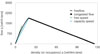 |
Fig. 1: traffic flow q as a function of traffic density k. |
Figure 1 shows a low density free flow phase, where speed is more or less homogeneous, and a high density congested phase where speeds vary. In the congested phase (as we all know), traffic alternately slows down and speeds up. The region on the road where speeds are low, typically moves upstream.
In practice, traffic quantities are measured using induction loops which are embedded in the road surface. To obtain macroscopic values, the quantities are averaged over time. Traffic flow is a simple count of vehicles, whereas occupancy (the proxy for density) is measured as the proportion of time the induction loops are covered (occupied) by a vehicle. Now, because occupancy increases with decreasing speed, the calculation of density isn’t entirely straightforward. This is because averaging traffic that is not in equilibrium isn’t straightforward. Let me explain this:
Usually, data represent 5 minute averages of observations, somewhere at a fixed point on the road. Now, 5 minutes is a long time period. We all know that five minutes in dense traffic can come with moments of free flow, speed decrease, stand still, speed increase and free flow again (if we are lucky). Hence, 5 minute averages during dense traffic usually are a complex mix of different types of traffic.
Further, it is relevant to point out that for these quantities there is no local equilibrium within the congested phase (“synchronised flow”), neither for driving observers nor for observers at a fixed point along the road. Traffic moves up and down the congested phase line. Mark that observers in a vehicle do not see the same behaviour as observers outside the vehicle, standing at a fixed point along the road. While drivers experience a decrease, a stand still and an increase, the stand still phase is completely missed by the roadside observer, who either sees one extremely slow vehicle which is actually standing still, or no vehicle at all, in case vehicles do not stand still directly above the induction loops. Knowing that induction loops with a vehicle above it for more than a few seconds reset itself and miss the vehicle as well, this shows that traffic that comes to a stand still is not correctly observed by induction loops. Hence, 5 minute averages of congested flow are constituted of very inhomogeneous traffic.
Figure 1 shows how flow decreases with density once density exceeds a specific critical value ρc. Essentially, this property: ρ>ρc is what causes the jam: The road cannot serve more than a specific maximum flow. This is because drivers do not accept less than some average minimum headway [time/vehicle]. This headway is essentially the reciprocal value of average maximum flow [vehicles/time]. When more vehicles enter the road at an on-ramp, and density exceeds the critical value, drivers need to decrease speed to maintain their (individual) accepted headway, and congestion arises… Of course, drivers who misbehave, e.g. by changing lanes suddenly or breaking suddenly, may also cause incidental congestion, but if flow is not yet at its critical value, the congested flow quickly dissolves again for obvious reasons.
Now, the most interesting phenomenon Andreas shows, is the upstream movement of the low speed wave. This wave is comparable to a sound wave in a moving gas, where particles slow down a little and form a temporary dense spot moving upstream. This upstream moving speed wave in traffic has a typical speed of -18km/h, a more or less uniform and constant value. And of course, this value is independent of the vehicle speed. This value of -18 km/h corresponds with the slope of the congested flow phase line (essentially a perfectly straight line!) in the phase diagram. However, due to the complex way density data are obtained from averaging 5 minute vehicle data, this straight line does not appear as such in a phase diagram based on averaged traffic data. Even if all vehicles would brake and accelerate in exactly the same pattern (one after the other), the averages would not show as a straight line due to averaging issues.
Moreover, averages of decelerating-only traffic would constitute a different congested flow line than accelerating traffic. This follows directly from the fact that decelerating vehicles with speed v0 pass the observation point at a lower speed than their predecessor, while for accelerating vehicles with exactly the same speed v0 it is the other way around: they drive faster than their predecessor at the observation point. This has consequences for the calculated averages of the traffic parameters.
With one induction loop, flow and occupancy can be measured, from which speed can be derived by means of formula [1]. Measuring speed directly is more accurate, as occupancy as measured is not the same as traffic density. Measuring speed, however, requires two induction loops for every lane at our observation point. However, measuring and averaging speed has a serious drawback when averaging is done incorrectly! The worst thing researchers can do is measure traffic speed directly and average this speed arithmetically! Although this is not a serious problem for free flow traffic, it is a serious drawback for congested traffic. The proper way to average speed is to apply the harmonic mean, as is explained in every standard textbook. Unfortunately in practice, this is often forgotten… There are several books on traffic theory, entirely and completely based on erroneously acquired data based on arithmetic speed averages. All this is also physics, and worth knowing!
In all: traffic congestion can be very well understood from the speed wave dynamics, but speed, flow and density measurements are very difficult to interpret directly due to averaging issues.
All Figures
|
Fig. 1: traffic flow q as a function of traffic density k. |
| In the text | |
Current usage metrics show cumulative count of Article Views (full-text article views including HTML views, PDF and ePub downloads, according to the available data) and Abstracts Views on Vision4Press platform.
Data correspond to usage on the plateform after 2015. The current usage metrics is available 48-96 hours after online publication and is updated daily on week days.
Initial download of the metrics may take a while.